
단변수 통계(2)
Chapter 03에서 배울 내용
- 주요 분포
- 모수적 검정 5가지
- 비모수적 검정 3가지
- 선형 모델
03 비모수적 검정
Spearman rank-order correlation(quantitative~quantitative)
Spearman 상관계수는 Pearson의 상관계수와 같다. 마찬가지로 -1과 1 사이의 값을 가게 된다. 다만 데이터가 정규분포를 따르지 않은 경우에 이용한다는 것이 다른 점이다.
import numpy as np
import scipy.stats as stats
import matplotlib.pyplot as plt

x = np.array([44.4, 45.9, 41.9, 53.3, 44.7, 44.1, 50.7, 45.2, 46, 47, 48, 60.1])
y = np.array([2.6, 3.1, 2.5, 5.0, 3.6, 4.0, 5.2, 2.8, 4, 4.1, 4.5, 3.8])

# Non-Parametric Spearman
cor, pval = stats.spearmanr(x, y)

# "Parametric Pearson cor test
cor, pval = stats.pearsonr(x, y)
Wilcoxon signed-rank test(quantitative ~ cte)
Wilcoxon signed-rank test(윌콕슨 부호 순위 검증)은 대응 표본의 전후 차이를 검증하는 방법으로 paired t-test에 해당한다. 먼저 전과 후에서 대응되는 데이터끼리의 차이의 절댓값을 이용하여 순위를 메긴다. 그 후, 각각의 차이에 대해 부호를 붙여 (+)와 (-)의 개수를 비교한다. 어떠한 개입이 유의하지 않았다면 (+)와 (-)의 개수가 비슷하겠지만, 유의했다면 둘의 차이는 클 것이다. 다만, 이 역시 데이터가 정규분포를 따르지 않을 때 사용한다. 민감도가 t-test보다 작기 때문에 샘플 사이즈가 너무 작다면 제대로 된 검정이 이루어지지 않을 수 있다. 귀무가설은 두 집단 사이의 평균에 차이가 없다는 것이다.
import numpy as np
import scipy.stats as stats
n = 20

bv0 = np.random.normal(loc = 3, scale = .1, size = n)
bv1 = bv0 + 0.1 + np.random.normal(loc = 0, scale = .1, size = n)

# Create an outlier
bv1[0] -= 10

print(stats.wilcoxon(bv0, bv1))
Mann-Whitney U test(quantiative~categorical(2 levels))
다른 말로 Mann-Whitney-Wilcoxon, 혹은 Wilcoxon rank-sum test(윌콕슨 순위합 검정)라고도 불린다. 이는 두 그룹의 평균이 같은지를 비교한다. 독립 t-test에 해당한다. 귀무가설은 역시나 두 그룹의 평균은 차이가 없다는 것이다.
import numpy as np
import scipy.stats as stats

n = 20

bv0 = np.random.normal(loc=1, scale=.1, size=n)
bv1 = np.random.normal(loc=1.2, scale=.1, size=n)

# create an outlier
bv1[0] -= 10

# Mann-Whitney U test
print(stats.mannwhitneyu(bv0, bv1))
04 선형 모델
선형 회귀 모델은 다음과 같은 식으로 표현됩니다. 개의 표본을 관측하였을 때 관측치인
와 독립변수인
에 관한 식으로 나타낼 수 있습니다.
Independent variable(독립 변수) 독립변수는 그 자체로 특정적인 값을 가지는 변수로 다른 변수들에 의해 변하지 않습니다. 예를 들어, 누군가의 나이는 독립변수가 될 수 있습니다. 그가 무엇을 먹는지, 텔레비전을 얼마나 보는지 등의 변인은 나이라는 변수의 값을 바꿀 수 없기 때문입니다. 만약 두 변수간의 관계를 본다 하다면, 그것은 독립변수가 다른 변수(종속 변수)에 영향을 주는지를 알아보는 것입니다.
Dependent variable(종속 변수) 종속변수는 다른 변수에 의해 영향을 받는 변수를 말합니다. 예를 들어, 시험 점수는 당신이 얼마나 공부를 열심히 했는지, 시험 전날 잠을 얼마나 잤는지 등의 변인에 의해 영향을 받습니다. 많은 경우에서 종속 변수에 영향을 미치는 변인이 무엇인지 파악하기 위해 애씁니다. 머신러닝에서는 이를 target variable이라고도 부릅니다.
단순 선형 회귀(Simple regression): test association between two quantitative variables
salary 데이터를 이용하여 Experience가 Salary에 미치는 영향을 알아봅시다.
import pandas as pd
import matplotlib.pyplot as plt

url = 'https://raw.github.com/neurospin/pystatsml/master/data/salary_table.csv'
salary = pd.read_csv(url)
1) Model the data
먼저 가설을 설정합니다.
Salary는 Experience의 선형함수로 표현된다.
the slope or coefficient or parameter of the model,
the intercept or bias is the second parameter of the model,
the
th error, or residual with
2) Fit: estimate the model parameters
Mean squared error(MSE) 혹은 Sum squared error(SSE)를 최소화시키는, 이른바 Ordinary Least Squares(OLS) 방법을 사용합니다.
from scipy import stats
import numpy as np
y, x = salary.salary, salary.experience
beta, beta0, r_value, p_value, std_err = stats.linregress(x,y)
print("y = %f x + %f, r: %f, r-squared: %f,\np-value: %f, std_err: %f"
% (beta, beta0, r_value, r_value**2, p_value, std_err))
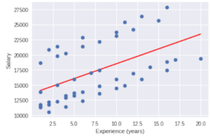
print("Regression line with the scatterplot")
yhat = beta * x + beta0 # regression line
plt.plot(x, yhat, 'r-', x, y,'o')
plt.xlabel('Experience (years)')
plt.ylabel('Salary')
plt.show()
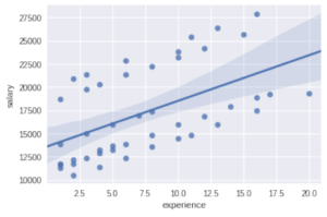
print("Using seaborn")
import seaborn as sns
sns.regplot(x="experience", y="salary", data=salary);
3) F-test
Goodness of fit 우선적으로 선형회귀 모델이 주어진 표본을 잘 설명해주는지를 판단합니다. 실제의 관측값과 모델을 통해 예측한 예상값의 차이를 살피는 것입니다. 여기서, 결정계수(explained variance)라 불리는 (R-squared)를 구하게 됩니다.
total sum of squares
sum of the sum of squares explained by the regression
sum of squares of residuals unexplained by the regression
다음으로, 를
의 분산의 측정치라고 합시다. 여기서 2는 intercept와 coefficient를 의미하며 이는 자유도에서 빠집니다.
Unexplained variance:
Explained variance:
Fisher 통계량은 위 두 가지 변수의 비율로 나타냅니다.